Open Street Map is considered a prominent example of volunteer geographic information (VGI). The community works based on collecting data from volunteer work and updating the database regularly. It is one of the largest opensource and free data providers in the world. Open Street Map was created by Steve Coast in UK (2004) and it was inspired by the success of Wikipedia. Because of the predominance of proprietary map data in the UK and everywhere in the world for that matter, the Open Street Map community was created, as an alternative to the commercial APIs of Google Maps, Bing Maps etc. The data is free for everybody, it doesn’t force the user to pay, the maps can be personalized by the user, in the way he wants, no adds or commercials are required. There are many ways in which the data from Open Street Map can be used. This paper presents one of them: building a tile server which will render tiles, in order to make beautiful maps. The studied area is Romania and we will concentrate on the mountainous regions of the country, by introducing hillshading and contour lines to the tiles.
Like in every open source community, there is a vast documentation about all the new developments, new software and tools and new trends. The “home” of the Open Street Map community on the World Wide Web is Github. Here are all the new tools published, one can find the largest collection of tutorials and documentation for the different tools and uses with OSM data. Almost all the important discoveries and discussions about the use of OSM are hosted here as well.
The project runs on Ubuntu 16.04, another open source, good documented operating system. The data was downloaded from www.geofabrik.de in *.osm.pbf format ("Protocolbuffer Binary Format"), which is primarily intended as an alternative to the XML format. It is about half of the size of a gzipped planet and about 30% smaller than a bzipped planet. It is also about 5 times faster to write than a gzipped planet and 6 times faster to read than a gzipped planet. The format was designed to support future extensibility and flexibility.The data was imported in a Postgresql database, which is the base of the project.
The OSM tile server stack is a collection of programs and libraries that work together to create a tile server. As so often with OpenStreetMap, there are many ways to achieve this goal and nearly all of the components have alternatives that have various specific advantages and disadvantages. The project is based on the standard version that is also used on the main OpenStreetMap.org tile server. It consists of 5 main components: Mod_tile, renderd, mapnik, osm2pgsql and a postgresql/postgis database. Mod_tile is an apache module, that serves cached tiles and decides which tiles need re-rendering – either because they are not yet cached or because they are outdated. Renderd provides a priority queueing system for rendering requests to manage and smooth out the load from rendering requests. Mapnik is the software library that does the actual rendering and is used by renderd.

After installing Ubuntu, some dependencies should also be installed:
sudo apt install libboost-all-dev git-core tar unzip wget bzip2 build-essential autoconf
libtool libxml2-dev libgeos-dev libgeos++-dev libpq-dev libbz2-dev libproj-dev munin-node munin
libprotobuf-c0-dev protobuf-c-compiler libfreetype6-dev libpng12-dev libtiff5-dev libicu-dev
libgdal-dev libcairo-dev libcairomm-1.0-dev apache2 apache2-dev libagg-dev liblua5.2-dev
ttf-unifont lua5.1 liblua5.1-dev libgeotiff-epsg
This list includes various utilities and libraries, the Apache web server, and “carto” which is used to convert Carto-CSS stylesheets into something that the map renderer can understand.
Postgresql is provides the database for the osm raw data. On Ubuntu, there are pre-packaged versions of both postgis and postgresql, so these can simply be installed via the Ubuntu package manager:
sudo apt-get install postgresql postgresql-contrib postgis postgresql-9.5-postgis-2.2
Here “postgresql” is the database for storing map data and “postgis” adds some extra graphical support to it. Now the postgis database needs to be created.On various tutorials, it is assumed that the name of the database is “gis”, so this name was used here also. It also requires a username and a password for the rendering account. The render account in this case is called “andreea”.
sudo -u postgres -I createuser andreea
createdb -E UTF8 -O andreea gis
“Sudo” allows a system administrator to give certain users the ability to run commands as “root”, “-u” does the actual installation of whatever program the user wants to install. With the command above we created the account for rendering and a database named “gis”. UTF-8 is a compromise character encoding that can be as compact as ASCII (if the ile is plain English text), buut can also contain any unicode characters (with some increase in file size). UTF means Unicode Transformation Format and 8 means that it uses 8-bit block to represent a character.
The database needs to be set up: the extensions need to be created at first with the command
CREATE EXTENSION postgis;
In postgis, it is required to set up the tables for the database: columns and rows, so the data for Romania will fit perfectly into the tables. The command is simple, a postgresql command, but in the Ubuntu command line environment:
ALTER TABLE geometry_columns OWNER TO renderaccount;
and
ALTER TABLE spatial_ref_sys OWNER TO renderaccount;
To import and manage the OpenStreetMap data into the database, osm2pgsql was used. This is a powerful command line-based program that actually converts raw osm data into the database.
mkdir ~/src # create a new directory “src”, where all the data will be stored later on.
# Src stands for “source”. It is the source of the server
>cd ~/src # move to the created directory
git clone git://github.com/openstreetmap/osm2pgsql.git
# download the latest version of the tool into this directory using the github link
cd osm2pgsql # a new directory “osm2pgsql” was created in src directory
The build mechanism used by osm2pgsql has changed since older versions, so there is a requirement to install more prerequisites for that:
sudo apt install make cmake g++ libboost-dev libboost-system-dev libboost-filesystem-dev
libexpat1-dev lib1g-dev libbz2-dev libpq-dev libgeos-dev libgeos++-dev libproj-dev lua5.2 liblua5.2-dev
Boost is a set of libraries for the C++ programming language that provide support for tasks and structures such as linear algebra, pseudorandom number generation, multithreading, image processing, regular expressions, and unit testing. It contains over eighty individual libraries.
The next command makes the installation of osm2pgsql:
sudo make install
Like already said in this paper, Mapnik is the library that does the actual rendering of the maps. There are many software libraries like Mapnik, but the authors chose this one because it is based on Python programming language and they are familiar with it. For this software, the latest version (Mapnik 2.2 – in May 2017 that was the latest version for Ubuntu) was used.
sudo apt-get install autoconf apache2-dev libtool libxml2-dev libbz2-dev libgeos-dev libgeos++-dev
libproj-dev gdal-bin libgdal1-dev libmapnik-dev mapnik-utils python-mapnik
This command installs the libraries for Mapnik, based on apache2 libraries. The software works together with gdal tool, which also provides libraries and dependencies for it.
To Install the tool takes a lot of time (hours in our case) and brings back lots of messages to the command line, so it is very time consuming to check for errors through these messages. To check if the tool is install correctly, it can be imported in python. If this will result in an error, then Mapnik is not correctly installed. If Mapnik is correctly installed, no error will appear, which means that Python can import it:
python #open Python in the Ubuntu command line
>>> import mapnik
>>> #no error message,means that Mapnik was found by Python
Mod_tile is the system that serves raster tiles. Renderd actually renders the tiles when mod_tile requests them. The two software were downloaded from Github.
The style that was used is the one used by the standard maps on the Open Street Map official site, which was modified for the contour lines and hillshading. This stylesheet is well documented and works everywhere in the world; for these reasons, it was chosen.
# download the stylesheet
git clone git://github.com/gravitystorm/openstreetmap-carto.git
sudo apt install npm nodejs-legacy # install node.js
sudo npm install -g carto # install Carto Map Stylesheet compiler
The downloaded stylesheet is in MML format, but Mapnik reads only XML formats. For this reason, a compiler (carto) needs to convert the original file in something that Mapnik can understand:
carto project.mml > mapnik.xml
The output from the command above is a Mapnik stylesheet named “mapnik.xml” in the same location as the input raw data.
The raw data (coordinates for all amenities and landcover) was downloaded from GeoFabrik. Here one can find raw data for the whole world, which is divided in continent/country sections. The format available for download is *.osm.pbf or zipped shapefiles. For the project, we need the file named romania-latest.osm.pbf. At the starting time of the project, it was last updated on 15th of May 2017, but since then it was several times updated; Geofabrik updates its data once a week, on Wednesdays.
The data was downloaded in this way:
mkdir ~/data # in the source folder/openstreetmap-carto, make a new directory called data
cd ~/data # navigate to the folder
wget http://download.geofabrik.de/europe/romania-latest.osm.pbf
#download the latest version of the raw data for Romania from Geofabrik. The output will be in *.osm.pbf format.
The next step is to load the data into the Postgis database, that was created in step 3.1. For this step, osm2pgsl is needed. This tool will import the data in the database, create way, nodes and relations out of the raw osm data. The following command was used in the Ubuntu command line:
osm2pgsql -d gis --create --slim -G --hstore --tag-transform-script ~/src/openstreetmap-carto/openstreetmap-carto.lua -C 2500 --number-processes 1 -S ~/src/openstreetmap-carto/openstreetmap-carto.style ~/data/romania-latest.osm.pbf
The database to work with is “gis”, that was created before, when installing PostgreSQL (-d gis in the command). The data is loaded now into an empty database (-create). When importing other data in the same database, the command will be -append.
Osm2pgsql can use different table layouts, but for rendering only “slim” tables work. The -G command determines how the multipolygons are processed. To allow tags for which there are no explicit database columns to be used for rendering, the - -hstore command was used. The script used for the tag process is “openstreetmap-carto.lua”. It is defined with the command - - tag-transform-script. This is an easy way to process OSM tags before the style itself processes them, making the style logic potentially much simpler.
For the import process 2.5 GB of memory were allocated to osm2pgsql (-C 2500). The command - - number-processes 1 allocates 1 CPU to the importing process. -S means creating the database columns in the input file (*.pbf). Now the data is loading and it takes a while, depending on the computer used and on the amount of data that is imported. In this case it took over 6 hours to load the data, because the raw data was big (a whole country). It made over 10 000 ways, 3 000 nodes and 4 000 relations.
Some shape files are still needed for the low-zoom country boundaries. They were downloaded and indexed using a python script from openstreetmap-carto. It takes considerable time when running the script to download all the shapefiles for all countries.
cd ~/src/openstreetmap-carto/ # the path where the python script is located
scripts/get-shapefiles.py # running the python script to get the needed shapefiles
Around the world, not all the places are written in Latin characters, but because Romania is using the a-z alphabet, there is no need to install other fonts than the default. It may be that at some point other data from around the world will be inserted in the same database, in order to create the same kind of elevation maps that are now created for Romania, so the fonts were however installed:
sudo apt-get install fonts-noto-cjk fonts-noto-hinted fonts-noto-unhinted ttf-unifont # extra fonts, beside the default ones
Renderd is the tool that renders the tiles so it needs a connection to the data that needs to be rendered, to the styles that we need to use and to a website where the tiles are displayed. It has a configuration file, where one should write the number of threads, the directory to which rendered tiles are going, the settings for Mapnik and an “ajt” section that makes the connection between the stylesheet and the rendering process (see Figure 1). This section actually corresponds to the named map style.
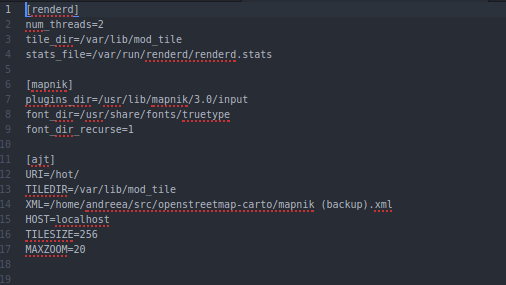
In this configuration file, the most important change that needs to be done is the location of the XML stylesheet. All the rest are set by default when installing Mapnik, Mod_tile and Renderd. The number of threads is set to 4 by default, but if the computer has less than 4 GB of memory (like in this case), the value should be changed to 2. If there are more styles on the map, one needs more map style sections on the configuration file of Renderd, but the URI should be different. In this case there is just one style section because only one style was used, with the URI “hot”, chosen so that the tiles generated can more easily be used in place of the HOT tile layer at OpenStreetMap.org. Of course, the URI name can be modified to choose another layer for the tile viewing.
In the configuration file of Apache2, a connection with Mod_tile needs to be made. The following line has been added in the file:
LoadModule tile_module /usr/lib/apache2/modules/mod_tile.so
After this, the configuration file needs to be ran, so it can process the changed line from above:
sudo a2enconf mod_tile
Another connection needs to be made between Apache and Renderd. For this the virtual host configuration file of Apache was modified. Virtual host files are the files that specify the actual configuration of the virtual hosts and dictate how the Apache web server will respond to various domain requests. Apache comes with a default virtual host file called “000-default.conf”. To this file the following lines were added between the ServerAdmin section and Document lines, in order to “tell” Apache about Renderd:
LoadTileConfigFile /usr/local/etc/renderd.conf
ModTileRenderdSocketName /var/run/renderd/renderd.sock
# Timeout before giving up for a tile to be rendered
ModTileRequestTimeout 0
# Timeout before giving up for a tile to be rendered that is otherwise missing
ModTileMissingRequestTimeout 30
After this, Apache needs to be reloaded twice:
sudo service apache2 reload
sudo service apache2 reload
Now, if a web browser is pointed to "http://server_ip_address/index.html" will result in the Ubuntu/Apache’s “It Works!” page (see Figure 2).
 of Apache's index file.png)
In order to start rendering tiles, the configuration file of Renderd needs to be run, first of all because some changes were made to this file and secondly because it is the first time when the rendering process is taking place on the server since the installation:
renderd -f -c /usr/local/etc/renderd.conf
***Note: this command needs to be done every time something is changing in the configuration file (e.g. when modifying the XML style sheet). In this way Renderd is ran in the foreground and all the errors (if there are any) will be shown on Ubuntu’s command line (e.g. errors from the style sheet). On a computer that has Ubuntu as the basic operating system, from here the rendering process starts without problems. On the other hand, if the server is set up on the virtual machine based on Ubuntu, one needs to reboot every time after running the above command. It might be because of the allocated resources to the virtual machine.
After this, if the browser is pointed at http://server_ip_address/hot/0/0/0.png, a map of the world is shown (see Figure 3).

To make this program start automatically every time, this should be set:
sudo systemctl enable renderd
To view the tiles, there are 2 possibilities: create a website connected to the server or use a website like OpenStreetMap.org to view the rendered tiles. This is more like “borrowing” the OpenStreetMap website to be able to see your tiles. For the presentation of the project, the second option was used at first. In a subsequent phase, a webpage was created for displaying the tiles created.
In a Google Chrome browser “Switcheroo Redirector” extension was installed (source: https://chrome.google.com/webstore/detail/switcheroo-redirector) and set up to take the rendered tiles from the server and bring them to the layer “Humanitarian” from OpenStreetMap.org. At the section “From” http://tile-a.openstreetmap.fr/hot/ was added, and at the “To” section the IP address of the server was typed in (see Figure 4).

Now, when pointing the browser to Romania's coordinates and switch to the Humanitarian layer, a map of the world will be displayed and Romania is the only country that appears on this map. This happens because in the server database just the data from Romania exists. (see Figure 5).
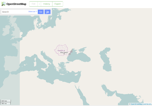
In the background Renderd is doing the rendering process, so whenever the map is zoomed in with focus on Romania, it creates new tiles (see Figure 6 for an example).
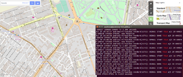
The purpose of the project is to create beautiful maps from the server, with contour lines and 3D effect, which can be seen especially in the Carpathian Mountains.
The data for the contour lines was downloaded from USGS – here SRTM (Shuttle Radar Topography Mission) data by the NASA is available. This is, in part of the world, available in 1 arc-second resolution (30m at the Equator), and in 3 arc-second resolution (90m at the Equator) for the whole world (below 60° latitude). Data for Romania can be found here.
The website provides raw DEM data in *.hgt format files that are compressed. The data is sectioned in tiles, according to latitude and longitude. For Romania 56 tiles were used: from N44E020 to N48E030.
After downloading, the data needs to be converted in the proper format. There is a popular script online that converts the SRTM HGT format into .tif format. It's basically a georeferenced image file with elevation data represented as different brightness values. The script can be found here (a preview and explanation are shown below. This is an adapted script for this project).
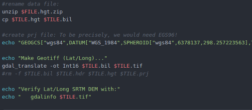
The bash file creates two of formats: *bil, and *.tif (GEOTIFF). The image format (tif) is the only one needed in the following steps. In order for the contour lines to appear on the map, they need to be on the server, but the database does not support raster images, so they need to be converted in a format that can be stored by PostgreSQL. Another option is to transform the tif image into shapefiles and store them in a folder on the computer, then modify the stylesheet for each set of contour lines and at the data source section (in the XML file) type the hardcoded location of the contour lines. We tried both possibilities, but without success so far.
First we need to make sure the reference system is specified in the file (which is not always the case):
for X in *.tif; do gdal_translate -of GTiff -co "TILED=YES" -a_srs "+proj=latlong" “$X” ; done
The image is warped in the next step in the Spherical Mercator Projection, because this is what Mapnik actually reads:
for X in *.tif: do gdalwarp -of GTiff -co "TILED=YES" -srcnodata 32767 -t_srs "+proj=merc +ellps=sphere +R=6378137 +a=6378137 +units=m" -rcs -order 3 -tr 30 30 -multi “$X”: done
For this step the gdal tool was used, which translates the image into a shapefile:
gdal_contour -i <step> -snodata 32767 -a height '<srtm.tif>' '<srtm.shp>'
For <step>, the elevation difference between adjacent contour lines, in the units used by the DEM was specified. In this case, this is meters. The -snodata option specifies the value used in the image tiles to denote missing elevation values (which is -32768 for current CIAT/CSI data). Now, the contour lines can be imported into the PostGIS database:
shp2pgsql <-c/-a/-d> -I -g way '<srtm-file without shp extension>' contours | psql -q <postgis db name>
Shp2pgsql is a tool that imports the shapefiles into the database. In this case a bash file was ran because of the big amount of data that we had. Every set of contour lines was imported in the database, using this script. The next step is to add styles for the contour lines in the stylesheet, so that Mapnik can read them and when rendering the tiles, they will be displayed on the map.
In the stylesheet, it is required to add the contour lines layers (56 in this case), where one wants them to appear - in this case after the landcover layers, so they will appear on top of them. The layers contain the style rules and the data source (where these layers are stored, where can the rendering program can find them). The first section that needs to be added is the style section, where the style rules are defined (see below):

The Maximum Denominator value represents the zoom level at which the contours can be seen. In the example above, the contours will be seen at zoom level 4 for the first time. We have tried different zoom levels, but the result is the same – the contour lines do not appear on the map. The Line symbolizer element defines the color and the width of every line. These values can be modified every time, it depends on the user’s preferences.
After the style rules are added to the XML file, the layer elements should also be added (an example is provided in the figure below):
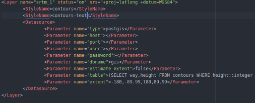
Every layer contains the style rules defined earlier and the source of the data (the gis database).
Since this method was not successful, we tried also the shapefile approach.
This method requires that the shapefiles remain on the computer (which acts like a server) and in the stylesheet the data source (the path where the files are stored) should be linked to each layer defined in the XML stylesheet, like shown below:

The path for the layer above is a folder that contains all the shapefiles. The layer above is one of the 10 m contours (we generated 10 m, 50 m and 100 m contour lines for each set of DEM).
This method was also not successful, even when changing the projection or adding the contour layers and styles as the first elements that should appear on the map. It might be to be a problem with the arrangement in the XML stylesheet, that was not noticed, even though more than enough time was spend dealing with this problem. This method works very good for the hillshading layers, but not for the contour lines.
The hillshading of the map was done from the georeferenced and warped images used in the contour lines step. It is a simple command from the Ubuntu’S terminal:
for X in *.tif; do gdal -hillshade “$X”; done
One of the resulting shaded images is presented below:
.png)
Like we did for the contour lines, we also need to define a style for the “hillshade layers” and add these layers to the XML stylesheet. Because these elements are raster formats, it is a difference in defining the styles and the layers have other properties than the contour lines (see figure below):
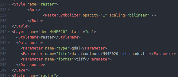
These layers were added as first layers and the following layers (just the ones that are actually polygons, like landcover elements) were set to a 50% opacity, so that the 3D effect is more visible. (the attribute for that is fill-opacity=”0.5”).
The rules for raster formats include the opacity (in this case it is set to 100%, so that the 3D effect will be more obvious) and the scaling which can be bilinear, fast and bilinear8. These Three options, defined by the XML Schema for Mapnik, define the interpolation method: bilinear uses the bilinear interpolation for all 4 channels (RGBA), bilinear8 assumes just one channel and fast uses the nearest neighbor. In this case the bilinear attribute was implemented.
The georeferenced files are stored on the computer, so the data source is the path where they are located. For a raster layer, the type and the format also need to be defined: they have the type set to gdal because this was the method used to create them and the format is tiff, of course.
**Note: It is recommended to run the configuration file of renderd after every modification of the stylesheet, so that eventual errors (most of the time they come from mistyping) can be detected. A performant text editor is also recommended. We used in thjis case Atom Editor (also open source).
After starting the rendering process and while the tiles are loaded at different zoom levels, the hillshade effect appears on the website:
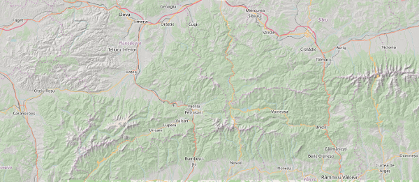
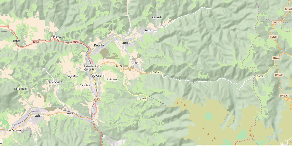
To make use of the created tiles, there are two possibilities: OpenLayers or Leaflet.
OpenLayers is the standard library for embedding an OpenStreetMap into a webpage. Leaflet, on the other hand, is a relatively new JavaScript library, but very well documented and easy to understand and to use. This was the preferred way to display the created tiles for this project.
Leaflet is available on Leaflet's homepage. To create the webpage, the Leaflet script was embedded in HTML. In the resulting map, Romania will be positioned in the center of the screen. The page is a sort of “Open Street Map”, only for one country, including hillshading effect. The following figure presents the Leaflet variables embedded in HTML.
Sequentially, other elements will be added to the website (e.g. a search bar) to make it more functional.
There are many tutorials for how to implement the architecture of a similar project (over 100, to be exact), but the idea behind them remains the same. This kind of project can be also implemented with a Windows operating system, but because OpenStreetMap community is a free open source, most of its members and users prefer to use only open source tools. Ubuntu is very well documented (e.g. every command line is explained on the askubuntu.org website, it doesn’t matter if the user never worked with it before, the answers are there). Also, there are many tools developed on github.com to help the user find the best solution for its project and they can be combined (we have combined at least 3 different tutorials, in order to get the expected result). Unfortunately, even though the open source community is so vast and everything is well documented, there are still some minor gaps in the implementation of the technologies used: some tools are complicated to use or to understand, other require sophisticated hardware and also, among so many possible solutions it is hard to find the perfect one.
Melanie Hofmann (HFT student) (2009): „Preparation of SRTM data for use as a worldwide digital terrain model “
Marc Rentschler (HFT student) (2012): „Generating tiles from existing hillshading raster data sets“
Christian Prägitzer (HFT student) (2010): „Conception and implementation of a GIS Architecture for documentation and decision support in catastrophe management“